
Normalization refers to the rescaling of real values to a common range, such as between 0 and 1. It is commonly used as a preprocessing technique in data processing and analysis.
Normalization in this context is the process of mapping data values to colors. Matplotlib provides various normalization techniques including:
The default behavior in Matplotlib maps colors linearly based on data values within a specified range using matplotlib.colors.Normalize().
import matplotlib as mpl
from matplotlib.colors import Normalize

norm = Normalize(vmin=-1, vmax=1)
normalized_value = norm(0)
print('Normalized Value', normalized_value)Uses colors.LogNorm(), ideal for wide-ranging values.
import matplotlib.pyplot as plt
import numpy as np
from matplotlib import colors

X, Y = np.meshgrid(np.linspace(-3, 3, 128), np.linspace(-3, 3, 128))
Z = (1 - X/2 + X**5 + Y**3) * np.exp(-X**2 - Y**2)

fig, ax = plt.subplots(1, 2, figsize=(7,4), layout='constrained')

pc = ax[0].imshow(Z**2 * 100, cmap='plasma', norm=colors.LogNorm(vmin=0.01, vmax=100))
fig.colorbar(pc, ax=ax[0], extend='both')
ax[0].set_title('Logarithmic Normalization')

pc = ax[1].imshow(Z**2 * 100, cmap='plasma', norm=colors.Normalize(vmin=0.01, vmax=100))
fig.colorbar(pc, ax=ax[1], extend='both')
ax[1].set_title('Linear Normalization')

plt.show()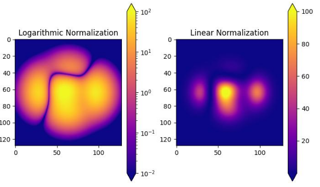
Use colors.CenteredNorm() to center your colormap around a value, useful for data with a meaningful zero point.
import matplotlib.pyplot as plt
import numpy as np
from matplotlib import colors, cm

X, Y = np.meshgrid(np.linspace(-3, 3, 128), np.linspace(-3, 3, 128))
Z = (1 - X/2 + X**5 + Y**3) * np.exp(-X**2 - Y**2)
cmap = cm.coolwarm

fig, ax = plt.subplots(1, 2, figsize=(7,4), layout='constrained')

pc = ax[0].pcolormesh(Z, cmap=cmap)
fig.colorbar(pc, ax=ax[0])
ax[0].set_title('Normalize')

pc = ax[1].pcolormesh(Z, norm=colors.CenteredNorm(), cmap=cmap)
fig.colorbar(pc, ax=ax[1])
ax[1].set_title('CenteredNorm()')

plt.show()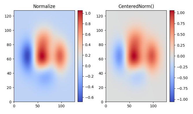
colors.SymLogNorm() handles both negative and positive values with logarithmic scaling.
import matplotlib.pyplot as plt
import numpy as np
from matplotlib import colors, cm

X, Y = np.mgrid[-3:3:complex(0, 128), -2:2:complex(0, 128)]
Z = (1 - X/2 + X**5 + Y**3) * np.exp(-X**2 - Y**2)

fig, ax = plt.subplots(1, 2, figsize=(7, 4), layout='constrained')

pcm = ax[0].pcolormesh(X, Y, Z, norm=colors.SymLogNorm(linthresh=0.03, linscale=0.03, vmin=-1.0, vmax=1.0, base=10), cmap='plasma', shading='auto')
fig.colorbar(pcm, ax=ax[0])
ax[0].set_title('SymLogNorm()')

pcm = ax[1].pcolormesh(X, Y, Z, cmap='plasma', vmin=-np.max(Z), shading='auto')
fig.colorbar(pcm, ax=ax[1])
ax[1].set_title('Normalize')

plt.show()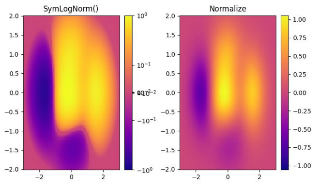
Uses colors.PowerNorm() for gamma-based transformation, useful for emphasizing different data regions.
import matplotlib.pyplot as plt
import numpy as np
from matplotlib import colors, cm

X, Y = np.meshgrid(np.linspace(-3, 3, 128), np.linspace(-3, 3, 128))
Z = (1 + np.sin(Y * 10.)) * X**2

fig, ax = plt.subplots(1, 2, figsize=(7, 4), layout='constrained')

pcm = ax[0].pcolormesh(X, Y, Z, norm=colors.PowerNorm(gamma=0.5), cmap='PuBu_r', shading='auto')
fig.colorbar(pcm, ax=ax[0])
ax[0].set_title('PowerNorm()')

pcm = ax[1].pcolormesh(X, Y, Z, cmap='PuBu_r', shading='auto')
fig.colorbar(pcm, ax=ax[1])
ax[1].set_title('Normalize')

plt.show()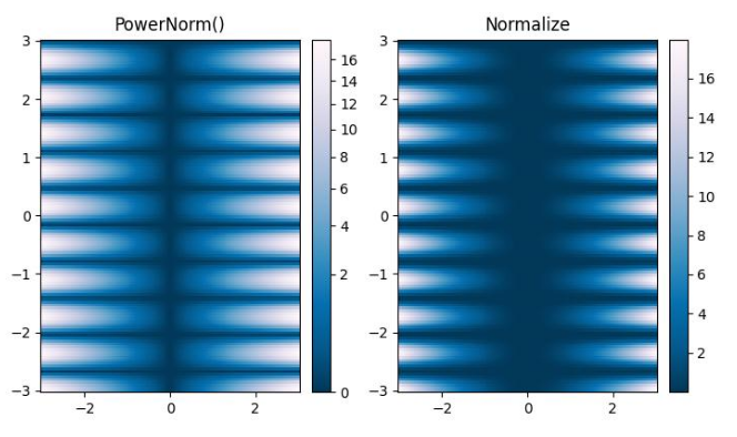
colors.BoundaryNorm() helps define specific boundaries with linearly distributed colors for segmented data visualization.
import matplotlib.pyplot as plt
import numpy as np
import matplotlib.colors as colors

X, Y = np.meshgrid(np.linspace(-3, 3, 128), np.linspace(-3, 3, 128))
Z = (1 + np.sin(Y * 10.)) * X**2

fig, ax = plt.subplots(2, 2, figsize=(7, 6), layout='constrained')
ax = ax.flatten()

pcm = ax[0].pcolormesh(X, Y, Z, cmap='RdBu_r')
fig.colorbar(pcm, ax=ax[0], orientation='vertical')
ax[0].set_title('Default norm')

bounds = np.linspace(-1.5, 1.5, 7)
norm = colors.BoundaryNorm(boundaries=bounds, ncolors=256)
pcm = ax[1].pcolormesh(X, Y, Z, norm=norm, cmap='RdBu_r')
fig.colorbar(pcm, ax=ax[1], extend='both', orientation='vertical')
ax[1].set_title('BoundaryNorm: 7 boundaries')

bounds = np.array([-0.2, -0.1, 0, 0.5, 1])
norm = colors.BoundaryNorm(boundaries=bounds, ncolors=256)
pcm = ax[2].pcolormesh(X, Y, Z, norm=norm, cmap='RdBu_r')
fig.colorbar(pcm, ax=ax[2], extend='both', orientation='vertical')
ax[2].set_title('BoundaryNorm: nonuniform')

bounds = np.linspace(-1.5, 1.5, 7)
norm = colors.BoundaryNorm(boundaries=bounds, ncolors=256, extend='both')
pcm = ax[3].pcolormesh(X, Y, Z, norm=norm, cmap='RdBu_r')
fig.colorbar(pcm, ax=ax[3], orientation='vertical')
ax[3].set_title('BoundaryNorm: extend="both"')

plt.show()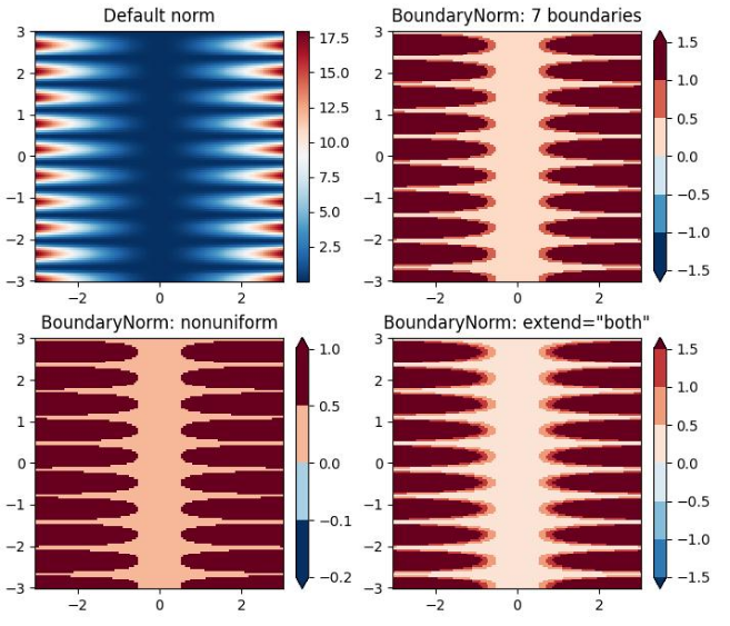
Advanced normalization like TwoSlopeNorm and FuncNorm can be used for further customization in special visualization scenarios. These are particularly useful in cases such as topography and oceanography or when needing full control over the mapping function.
This concludes the in-depth guide to colormap normalization in Matplotlib from Vista Academy.